Systat Confidence Bands

Grafiti LLC

Confidence Bands

Confidence Intervals & Confidence Bands

Basics

Sometimes we are asked how to get confidence intervals in linear models in Grafiti. It is actually not very hard and, here, we shall review the technique. Before we do, however, let’s review the basic ideas behind a confidence interval for a linear model.

First, if we have a linear regression of Y on the variable X, then we are actually saying that, for a given value of X, the value of Y is given by Y=aX+b+e where e is a “noise term.”

The noise term is usually assumed to be normally distributed with a mean of 0 and a variance of s^2. The trick for a real data set is to estimate a and b and then to carry out inferences on those estimates using an estimated value of s^2.

Sometimes, however, we would like to find a confidence interval for the mean of Y at a specified value of X. According to the equation above, the mean of Y at X is aX+b.

However, in a real data set, we never know the “true” values of a and b; all we know are our estimates. Therefore, it is appropriate to find an interval in which we can be relatively confident the true mean of Y occurs.

There are some very messy formulae for calculating this interval but we shall not go into them here. After all, the computer should make the computation easy. So, suppose we take the sample data set USSTATES.SYD, with 48 valid cases for the variables CARDIO and CANCER. Use the Statistics > Regression > Linear dialog box to set up the regression model or issue the commands:

REGRESS
USE usstates
SAVE regress/MODEL
MODEL cancer=CONSTANT+cardio
ESTIMATE

The computer will then estimate the model, finding estimated values for both the constant and the coefficient of CARDIO and printing out an analysis of variance table.

In this instance it will also save a file, REGRESS.SYD, that contains the residuals from the model, estimates of CANCER based on CARDIO for the model (the variable named ESTIMATE) and a mysterious value called SEPRED. It is SEPRED that we will use to calculate our confidence intervals.

SEPRED stands for “Standard Error of the Predicted Value. The file will also have the values of the original data. These are saved because we added the MODEL option to the SAVE command.

To calculate the UPPER and LOWER limits of a 95% confidence interval for the predicted values of CANCER, use the Data > Transform > Let dialog box or enter the BASIC module and issue the commands:
BASIC
USE regress
LET n=48
LET nvars=2
LET upper = estimate+TIF(.975,n-nvars)*sepred
LET lower = estimate-TIF(.975,n-nvars)*sepred
PRINT upper lower
RUN

The UPPER and LOWER confidence limits for the estimated value of CANCER for each case will then be printed out. In the above, TIF stands for the “Inverse t-distribution.”

The above ideas can be generalized in several different ways. For example, if you wish to find a confidence interval for the mean of Y for a regression on two variables, you only need to add those variables to the MODEL statement in REGRESS and change NVARS from 2 to 3 in the BASIC module. (Note: N-NVARS represents the number of valid cases minus the number of variables in the model. Set N and NVARS above to the correct number of cases and variables for your model.

Confidence Intervals for the Mean of Y at New Values of X

It may happen that you wish to find the confidence interval for the mean of Y at one or more new values of your X variable. Put the new values of X at the end of your file and make the associated Y values zero. (You don’t need to worry about what the Y-value actually is. This Y-value is just a placeholder and will not enter into the calculations.)

Next, add a new variable in your file called WT. WT should have the value 1 for the cases on which you have data for both X and Y, and 0 for the cases with new values of X. After saving the file, use the Data > Frequency dialog to select WT as your weighting variable, or issue the command:

FREQUENCY=WT

Using the Statistics > Regression > Linear dialog box or a command file, estimate your regression model again, remembering to save the results to a data file with MODEL option. The FREQUENCY command is very useful in this context; in calculating the regression, points with weight 1 will be used once, points with weight zero will be used zero times.

Thus, the regression will be calculated for the cases with known values of Y and X. However, the value of ESTIMATE will be calculated for all cases. Using the file of saved results, you can use the calculation above to derive the confidence interval for the estimated mean of an unknown Y at a known value of X for the new cases.

Subtleties

There are a couple of subtleties concerning this type of confidence interval that you should note. First, this is an interval for the mean of Y at a particular value of X, not a confidence interval or band for the regression line. If you plot the UPPER and LOWER confidence limits you will see two curving lines around the regression line. Returning to the original example using the USSTATES.SYD file, calculate the confidence interval values and plot: BEGIN PLOT cancer*x(1) /SIZE=0 SMOOTH=LINEAR SHORT YMIN=100 YMAX=300 , XMIN=100 XMAX=500 XLABEL=’CARDIO’ COLOR=BLUE PLOT upper,lower*x(1) /SIZE=0 SMOOTH=SPLINE SHORT YMIN=100 YMAX=300, XMIN=100 XMAX=500 YLABEL=’ ‘ XLABEL=’ ‘ COLOR=RED, OVERLAY END (In saving the results of the estimated model, SYSTAT renames the independent variables X(1). . . X(n), so that CARDIO is renamed X(1) in this example.)

It is tempting to think that these lines form a confidence band for the entire line. That is not true. The problem is that the upper and lower confidence limits are calculated by using one point at a time. In order to calculate a confidence band or interval for an entire line, we need to take into account the fact that two parameters, the constant and the coefficient of X, are being calculated for that line. Therefore, upper and lower confidence bands for the entire line would be given by: BASIC LET n=48 LET nvars=2 LET upperband = estimate+SQRT(2*FIF(.95,2,n-nvars))*sepred LET lowerband = estimate+SQRT(2*FIF(.95,2,n-nvars))*sepred PRINT upperband lowerband RUN

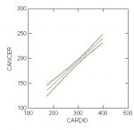
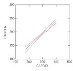
When you plot the confidence intervals for the estimated values of CANCER and the confidence bands for the regression line, you’ll see that the confidence band is wider than the confidence interval: BEGIN PLOT cancer*x(1) / SIZE=0 SMOOTH=LINEAR SHORT YMIN=100 YMAX=300 , XMIN=100 XMAX=500 XLABEL=’CARDIO’ COLOR=BLUE PLOT upper,lower*x(1) /SIZE=0 SMOOTH=SPLINE SHORT YMIN=100, YMAX=300 XMIN=100 XMAX=500 YLABEL=’ ‘, XLABEL=’ ‘ COLOR=RED OVERLAY PLOT upperband,lowerband*x(1) /SIZE=0 SMOOTH=SPLINE SHORT, YMIN=100 YMAX=300 XMIN=100 XMAX=500 YLABEL=’ ‘, XLABEL=’ ‘ COLOR=GREEN OVERLAY END

Because the relationship of CANCER (deaths per 100000 due to cancer) and CARDIO (deaths per 100000 due to cardiovascular disease) is linear, the difference between the confidence intervals for estimated values of CANCER and the confidence bands for the regression line is small, but even with well behaved data such as this the difference is apparent. Second, it is also tempting to think that 95% of all of the observations should fall within the confidence bands. This is also not true. These are confidence bands for the mean only. If you wish to find confidence bands for observations, you must modify the calculation as you see below. BASIC LET n=48 LET nvars=2 LET s_square=177.065 LET upperband = estimate+TIF(.975,n-nvars)*SQR(sepred^2+s_square) LET lowerband = estimate-TIF(.975,n-nvars)*SQR(sepred^2+s_square) PRINT upperband lowerband RUN

where S_SQUARE is the mean square residual from the regression. These are sometimes called prediction intervals. When entering your values for N and NVARS, also enter the value for S_SQUARE, which you will find in the Analysis of Variance table of the regression output. Now, if you wish to see the results of this calculation, issue the following command sequence:

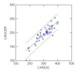
BEGIN PLOT cancer*x(1) /SMOOTH=LINEAR SHORT YMIN=100 YMAX=300 XMIN=100, XMAX=500 XLABEL=’CARDIO’ COLOR=BLUE PLOT upperband,lowerband*x(1) / SIZE=0 SMOOTH=SPLINE SHORT, YMIN=100 YMAX=300 XMIN=100 XMAX=500 YLABEL=’ ‘, XLABEL=’ ‘ COLOR=GREEN OVERLAY END This will plot the confidence bands or prediction intervals around the data.